Visualizing The Affects of Climate Change

Introduction

The study of climate change has been widely explored in the past few decades due it’s growing affect on our planet. From the rise of sea levels, carbon admission, and rising global temperatures, the change in our climate has had astounding effects on all terrestrial ecosystems. Changes in our atmosphere as early as the middle 1700’s has affected agricultural production globally across time and will continue to affect agricultural production for years to come. That being said our project Visualizing The Effects of Climate Change: Cases Studies in Africa is designed to map these changes in global temperature, precipitation, and crop yields as far back as possible. This project extends the work of scholars Andrew Challinor, Tim Wheeler, Chris Garforth, Peter Craufurd, and Amir Kassam which you can find here. Although this particular article will talk about specific crop yields across the African continent, our methods in data visualization and machine learning is prepared to tackle other regions of the world across time.

Methods

There are a few key components to understand Linear Regression(LR) vs Multiple Linear Regression(MLR). We will first talk about what exactly a “regression” is and its purpose. Then we will discuss the importance of Multiple Linear Regression for certain research questions.

Linear regression is a type of supervised learning algorithm. In order to understand this performance, you have to choose a performance measure or make up your own, a fitness function and/or cost function (Aurélien Géron 2017). For the sake of this project, we are using a cost function. A cost function determines how bad your model is, which is determined by the average “loss” over the entire training dataset. We used a cost function measure to observe the difference in the performance of our model as we added new parameters, which we added more parameters as different slopes in MLR and added rainfall data. Training data is data used in the training process, the training process is when we calculate our best LR or MLR model using the least-squares regression cost function.

One of the purposes of a machine learning model is to find patterns in data to make accurate predictions. This model is data-driven and mathematically informed. We will get into what some of those informative mathematical equations/measures are a little later. That being said, you can determine the accuracy of the model by calculating the difference between the training data and the regression line. The goal of the least-squares regression that we employ to decrease the sum of the distances between the predicted and observed response variables. Furthermore, there are two variables that are significant in describing a regression line. The two variables are called a response variable and an explanatory variable. Your response variable is typically represented by y and your explanatory variable is represented by X. X for an MLR can also be a multi-dimensional array, compared to your y, which is always one dimensional. A regression line basically describes the changes in your response variable when your explanatory variable changes Let’s look at an example of this using one of our visualizations.

Cassava: LR(left) vs MLR(right)

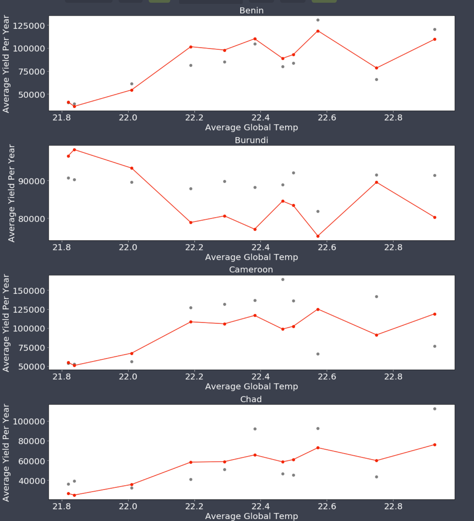
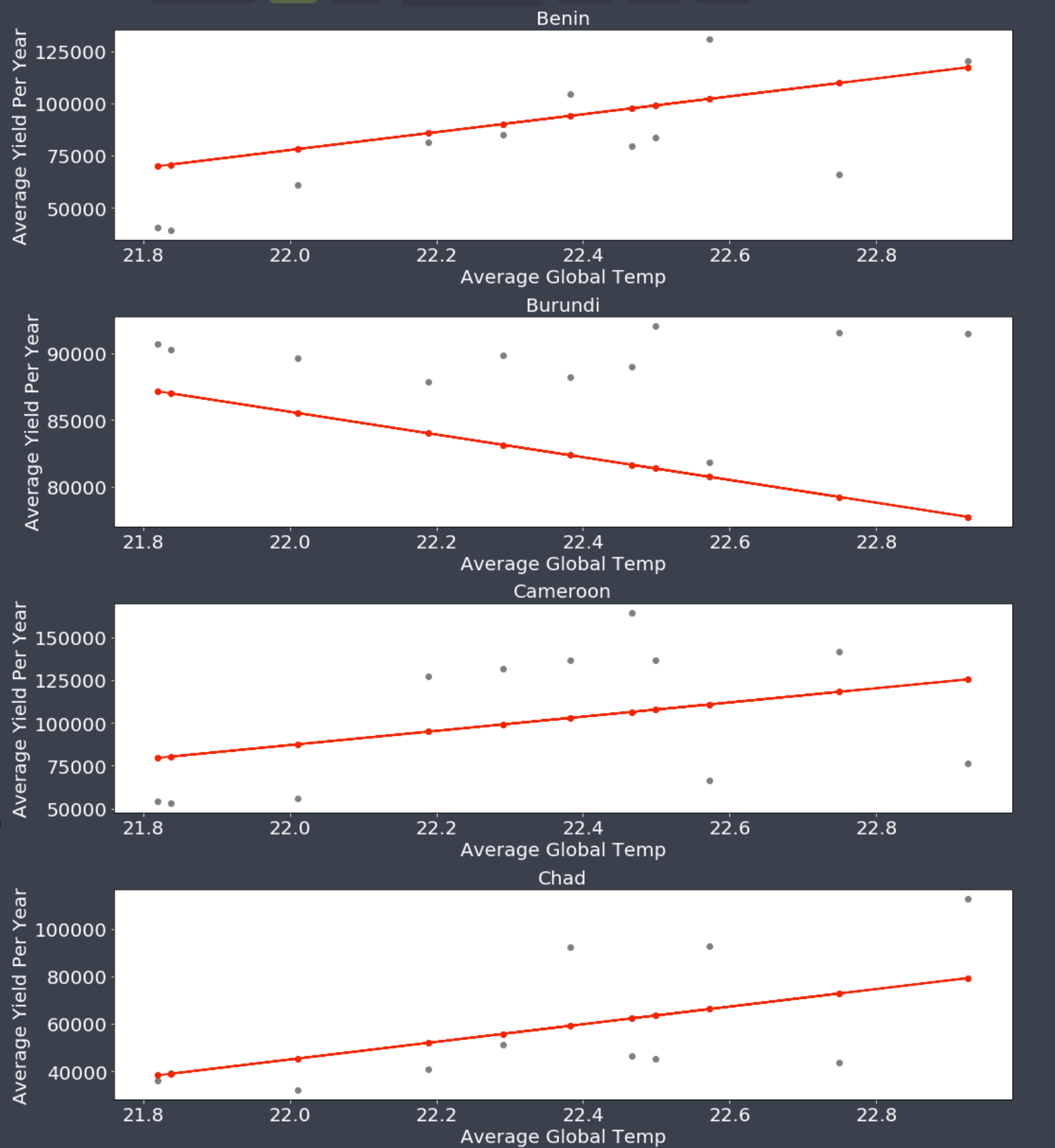
If you look at the above visualization for the crop cassava, on the left you have a linear regression model using only temperature as an explanatory variable, while on the right we show a multiple linear regression model which includes both temperature and precipitation as explanatory variables. The only difference between the left and right is the training data which adds precipitation data to our MLR. The linear regression has been created by training our algorithm using crop yields in a specified country for a specific year in global temperature and precipitation data. As you can see the model’s predictions are different between our LR and MLR model due to the inclusion of precipitation data.

In regression models, several measures of “goodness of fit” are often discussed. Here we mention the three most common - mean square error (MSE), mean absolute error (MAE) and root mean square error (RMSE) (Aurélien Géron 2017). Our results are showed to the right while below are the differences between all three measures.

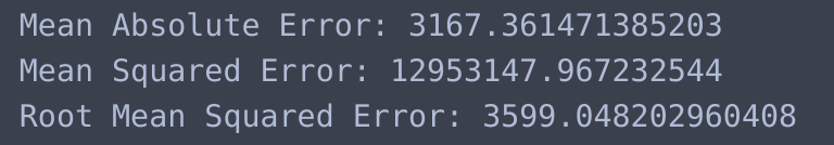
Mean Squared Error (MSE): Measures the average of error squares i.e. the average squared difference between the estimated values and true value.(Aurélien Géron 2017)

Mean Absolute Error (MAE): The average of the difference between predicted and actual values in the test, i.e. the average prediction error. (Aurélien Géron 2017)

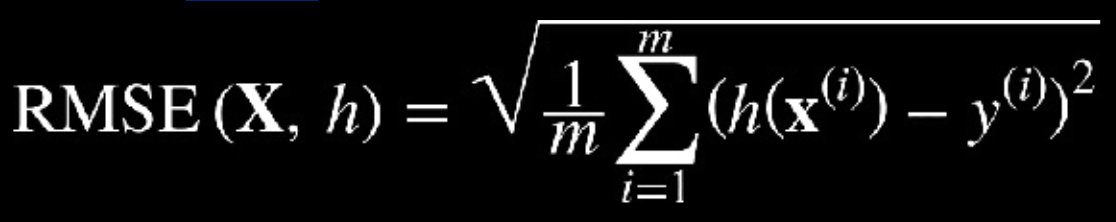
Root Mean Squared Error (RMSE): is the standard deviation of the residuals (prediction errors). Residuals are a measure of how far from the regression line data points are; RMSE is a measure of how to spread out these residuals are. (Aurélien Géron 2017)

Often times the loss function and cost function are used interchangeably although they technically calculate different things. Earlier we stated that the cost function is used to calculate the average loss over the entire dataset. Often the loss function is defined to calculate a single loss in a training data point. That being said, there are different loss functions. A loss function is a method to evaluate how your algorithm models your dataset. It’s able to do this by measuring the (distance/difference) between our observed y and our predicted y. The resulting value of that difference is referred to as a residual. If the output of the loss function is high that means your predictive value is off. On the other hand, if your output is low that means that your predictive value is good.

The dataset that we used for precipitation was gathered by the Global Precipitation Climogotoly Center which collects the monthly land-surface precipitation using rain gauges built on GTS data as well as historical data. The precipitation data that was gathered varies depending on time, calculated by months, longitude and latitude, which is particular to each country, and rainfall over a given month. Much of the cleaning, analyzing, and aggregation process had to do with calculating monthly measurements and organizing those monthly measurements into yearly measurements based on country. Our goal for our precipitation is to decrease the number of missing values for each country by increasing the resolution of the data. Currently, we are using a 2.5 resolution, we plan on using a 0.5 resolution for better accuracy.

Discussion

Although we’ve created a model our model fails to take into account all potential variables that could affect the change in climate in Africa. There seems to be some association between crop yields, temperature, and precipitation rates in a given country however we don’t have anything about causality. Also, we are using a simple two-parameter mlr model which can be more effective by adding more parameters. Therefore our model is not perfect and definitely needs some work. Here is a list of 5 “next steps” we plan on taking to address the shortcomings of our model in future research, accompanied by a brief explanation.

We plan on updating our temperature dataset with a more technical resource.

• Currently, we are using a temperature dataset from Kaggle, which is not ideal for our future work. We believe that by incorporating a dataset from a more technical resource we increase the accuracy of our temperature variable.

We plan on fitting a polynomial regression to understand how rainfall changes over the year

• This may give us insight into how extreme weather events such as droughts and floods affect crop production during particular parts of the year.

We plan on using more regional designations instead of countries.

• Do to both the size of the African continent as well as it’s colonial history, we plan on using more regional geographic designations in order to explore the changes in crop production based on a series of social and environmental variables. We believe it is important to understand how socio-political issues impact crop production.

Our knowledge of the science of African Climate Change is limited. Therefore we plan on doing more research into how other scholars in the field have gone about developing models to describe how Africa has been affected by climate change.

• Figure out Interactive Plot for Globes and Crops.

• Figure out how to output the data into a JSON file.

• Making the globes into a drop-down to select for different crops.

• Make the regression plots interactive.

• Create a Visual Design for Web Page.